18 KiB
- Object Detection
- Training & Class Imbalance
- RetinaNet architecture
- Feature Pyramid Network
- Anchors & Region Proposals
- Training
- Inference
- References
— title: Explaining RetinaNet author: Chris Hodapp date: December 13, 2017 tags: technobabble —
A paper came out in the past few months, Focal Loss for Dense Object Detection, from one of Facebook's teams. The goal of this post is to explain this paper as I work through it, through some of its references, and one particular implementation in Keras.
Object Detection
"Object detection" as it is used here refers to machine learning models that can not just identify a single object in an image, but can identify and localize multiple objects, like in the below photo taken from Supercharge your Computer Vision models with the TensorFlow Object Detection API:
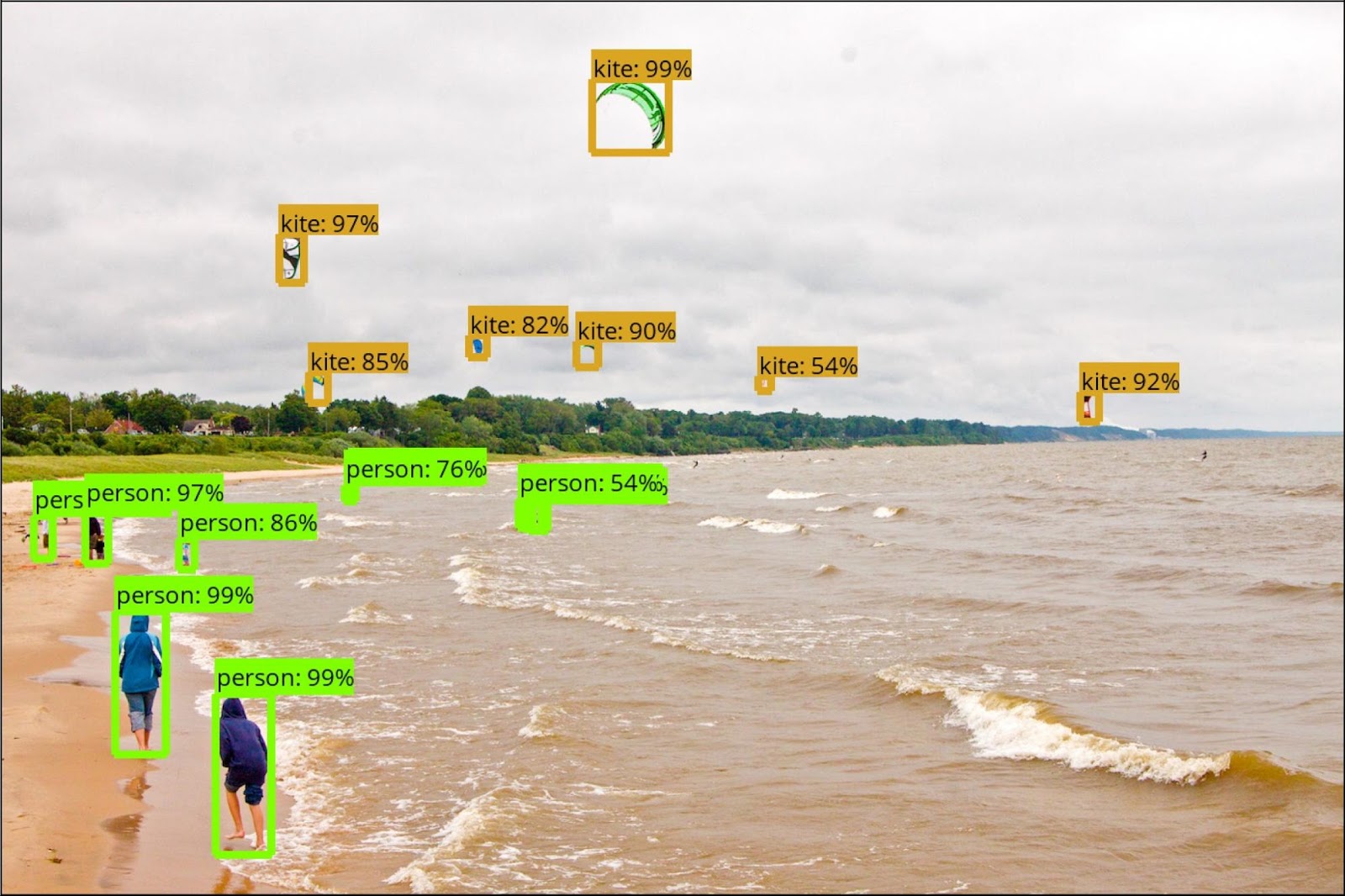
At the time of writing, the most accurate object-detection methods were based around R-CNN and its variants, and all used two-stage approaches:
- One model proposes a sparse set of locations in the image that probably contain something. Ideally, this contains all objects in the image, but filters out the majority of negative locations (i.e. only background, not foreground).
- Another model, typically a CNN (convolutional neural network), classifies each location in that sparse set as either being foreground and some specific object class (like "kite" or "person" above), or as being background.
Single-stage approaches were also developed, like YOLO, SSD, and OverFeat. These simplified/approximated the two-stage approach by replacing the first step with brute force. That is, instead of generating a sparse set of locations that probably have something of interest, they simply handle all locations, whether or not they likely contain something, by blanketing the entire image in a dense sampling of many locations, many sizes, and many aspect ratios.
This is simpler and faster - but not as accurate as the two-stage approaches.
Methods like Faster R-CNN (not to be confused with Fast R-CNN… no, I didn't come up with these names) merge the two models of two-stage approaches into a single CNN, and exploit the possibility of sharing computations that would otherwise be done twice. I assume that this is included in the comparisons done in the paper, but I'm not entirely sure.
Training & Class Imbalance
Briefly, the process of training these models requires minimizing some kind of loss function that is based on what the model misclassifies when it is run on some training data. It's preferable to be able to compute some loss over each individual instance, and add all of these losses up to produce an overall loss. (Yes, far more can be said on this, but the details aren't really important here.)
This leads to a problem in one-stage detectors: That dense set of locations that it's classifying usually contains a small number of locations that actually have objects (positives), and a much larger number of locations that are just background and can be very easily classified as being in the background (easy negatives). However, the loss function still adds all of them up - and even if the loss is relatively low for each of the easy negatives, their cumulative loss can drown out the loss from objects that are being misclassified.
That is: A large number of tiny, irrelevant losses overwhelm a smaller number of larger, relevant losses. The paper was a bit terse on this; it took a few re-reads to understand why "easy negatives" were an issue, so hopefully I have this right.
The training process is trying to minimize this loss, and so it is mostly nudging the model to improve where it least needs it (its ability to classify background areas that it already classifies well) and neglecting where it most needs it (its ability to classify the "difficult" objects that it is misclassifying).
This is class imbalance in a nutshell, which the paper gives as the limiting factor for the accuracy of one-stage detectors. While the existing approaches try to tackle it with methods like bootstrapping or hard example mining, the accuracy still is lower.
Focal Loss
So, the point of all this is: A tweak to the loss function can fix this issue, and retain the speed and simplicity of one-stage approaches while surpassing the accuracy of existing two-stage ones.
At least, this is what the paper claims. Their novel loss function is called Focal Loss (as the title references), and it multiplies the normal cross-entropy by a factor, $(1-p_t)^\gamma$, where $p_t$ approaches 1 as the model predicts a higher and higher probability of the correct classification, or 0 for an incorrect one, and $\gamma$ is a "focusing" hyperparameter (they used $\gamma=2$). Intuitively, this scaling makes sense: if a classification is already correct (as in the "easy negatives"), $(1-p_t)^\gamma$ tends toward 0, and so the portion of the loss multiplied by it will likewise tend toward 0.
RetinaNet architecture
The paper gives the name RetinaNet to the network they created which incorporates this focal loss in its training. While it says, "We emphasize that our simple detector achieves top results not based on innovations in network design but due to our novel loss," it is important not to miss that innovations in: they are saying that they didn't need to invent a new network design - not that the network design doesn't matter. Later in the paper, they say that it is in fact crucial that RetinaNet's architecture relies on FPN (Feature Pyramid Network) as its backbone. As far as I can tell, the architecture's use of a variant of RPN (Region Proposal Network) is also very important.
I go into both of these aspects below.
Feature Pyramid Network
Another recent paper, Feature Pyramid Networks for Object Detection, describes the basis of this FPN in detail (and, non-coincidentally I'm sure, the paper shares 4 co-authors with the paper this post explores). The paper is fairly concise in describing FPNs; it only takes it around 3 pages to explain their purpose, related work, and their entire design. The remainder shows experimental results and specific applications of FPNs. While it shows FPNs implemented on a particular underlying network (ResNet, mentioned below), they were made purposely to be very simple and adaptable to nearly any kind of CNN.
To begin understanding this, start with image pyramids. The below diagram illustrates an image pyramid:
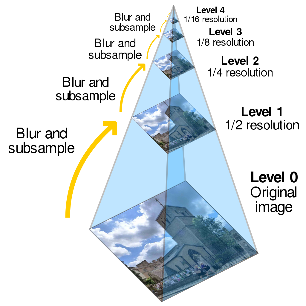

Image pyramids have many uses, but the paper focuses on their use in taking something that works only at a certain scale of image - for instance, an image classification model that only identifies objects that are around 50 pixels across - and adapting it to handle different scales by applying it at every level of the image pyramid. If the model has a little flexibility, some level of the image pyramid is bound to have scaled the object to the correct size that the model can match it.
Typically, though, detection or classification isn't done directly on an image, but rather, the image is converted to some more useful feature space. However, these feature spaces likewise tend to be useful only at a specific scale. This is the rationale behind "featurized image pyramids", or feature pyramids built upon image pyramids, created by converting each level of an image pyramid to that feature space.
The problem with featurized image pyramids, the paper says, is that if you try to use them in CNNs, they drastically slow everything down, and use so much memory as to make normal training impossible.
However, take a look below at this generic diagram of a generic deep CNN:
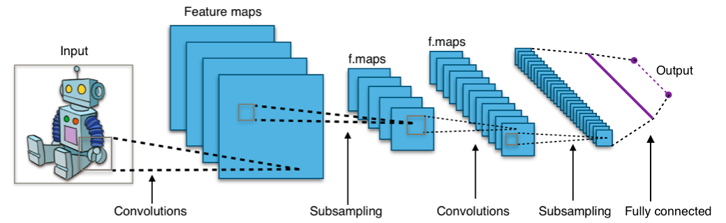

You may notice that this network has a structure that bears some resemblance to an image pyramid. This is because deep CNNs are already computing a sort of pyramid in their convolutional and subsampling stages. In a nutshell, deep CNNs used in image classification push an image through a cascade of feature detectors or filters, and each successive stage contains a feature map that is built out of features in the prior stage - thus producing a feature hierarchy which already is something like a pyramid and contains multiple different scales. (Being able to train deep CNNs to jointly learn the filters at each stage of that feature hierarchy from the data, rather than engineering them by hand, is what sets deep learning apart from "shallow" machine learning.)
When you move through levels of a featurized image pyramid, only scale should change. When you move through levels of a feature hierarchy described here, scale changes, but so does the meaning of the features. This is the semantic gap the paper references. Meaning changes because each stage builds up more complex features by combining simpler features of the last stage. The first stage, for instance, commonly handles pixel-level features like points, lines or edges at a particular direction. In the final stage, presumably, the model has learned complex enough features that things like "kite" and "person" can be identified.
The goal in the paper was to find a way to exploit this feature hierarchy that is already being computed and to produce something that has similar power to a featurized image pyramid but without too high of a cost in speed, memory, or complexity.
Everything described so far (none of which is specific to FPNs), the paper calls the bottom-up pathway - the feed-forward portion of the CNN. FPN adds to this a top-down pathway and some lateral connections.
Top-Down Pathway
Lateral Connections
As Applied to ResNet
For two reasons, I don't explain much about ResNet here. The first is that residual networks, like the ResNet used here, have seen lots of attention and already have many good explanations online. The second is that the paper claims that the underlying network
Deep Residual Learning for Image Recognition Identity Mappings in Deep Residual Networks
Anchors & Region Proposals
Recall last section what was said about feature maps, and the that the deeper stages of the CNN happen to be good for classifying images. While these deeper stages are lower-resolution than the input images, and while their influence is spread out over larger areas of the input image (that is, their receptive field is rather large due to each stage spreading it a little further), the features here still maintain a spatial relationship with the input image. That is, moving across one axis of this feature map still corresponds to moving across the same axis of the input image.
RetinaNet's design draws heavily from RPNs (Region Proposal Networks) here, and here I follow the explanation given in the paper Faster R-CNN: Towards Real-Time Object Detection with Region Proposal Networks. I find the explanations in terms of "proposals", of focusing the "attention" of the neural network, or of "telling the neural network where to look" to be needlessly confusing and misleading. I'd rather explain very plainly how they work.
Central to RPNs is anchors. Anchors aren't exactly a feature of the CNN. They're more a property that's used in its training and inference.
In particular:
- Say that the feature pyramid has $L$ levels, and that level $l+1$ is half the resolution (thus double the scale) of level $l$.
- Say that level $l$ is a 256-channel feature map of size $W \times H$ (i.e. it's a tensor with shape $W \times H \times 256$). Note that $W$ and $H$ will be larger at lower levels, and smaller at higher levels, but in RetinaNet at least, always 256-channel samples.
- For every point on that feature map (all $WH$ of them), we can identify a corresponding point in the input image. This is the center point of a broad region of the input image that influences this point in the feature map (i.e. its receptive field). Note that as we move up to higher levels in the feature pyramid, these regions grow larger, and neighboring points in the feature map correspond to larger and larger jumps across the input image.
- We can make these regions explicit by defining anchors - specific rectangular regions associated with each point of a feature map. The size of the anchor depends on the scale of the feature map, or equivalently, what level of the feature map it came from. All this means is that anchors in level $l+1$ are twice as large as the anchors of level $l$.
The view that this should paint is that a dense collection of anchors covers the entire input image at different sizes - still in a very ordered pattern, but with lots of overlap. Remember how I mentioned at the beginning of this post that one-stage object detectors use a very "brute force" method?
My above explanation glossed over a couple things, but nothing that should change the fundamentals.
- Anchors are actually associated with every 3x3 window in the anchor map, not precisely every point, but all this really means is that it's "every point and its immediate neighbors" rather than "every point". This doesn't really matter to anchors, but matters elsewhere.
- It's not a single anchor per 3x3 window, but 9 anchors - one for each of three aspect ratios (1:2, 1:1, and 2:1), and each of three scale factors ($1, 2^{1/3}, and 2^{2/3}$) on top of its base scale. This is just to handle objects of less-square shapes and to cover the gap in scale in between levels of the feature pyramid. Note that the scale factors are evenly-spaced exponentially, such that an additional step down wouldn't make sense (the largest anchors at the pyramid level below already cover this scale), and nor would an additional step up (the smallest anchors at the pyramid level above already cover it).
Here, finally, is where actual classification and regression come in. The classification subnet and box regression subnet are here.
Classification Subnet
Every anchor associates an image region with a 3x3 window (i.e. a 3x3x256 section - it's still 256-channel). The classification subnet is responsible for learning: do the features in this 3x3 window, produced from some input, image indicate that an object is inside this anchor? Or, more accurately: For each of $K$ object classes, what's the probability of each object (or just of it being background)?
Box Regression Subnet
The box regression subnet takes the same input as the classification subnet, but tries to learn the answer to a different question. It is responsible for learning: what are the coordinates to the object inside of this anchor (assuming there is one)? More specifically, it tries to learn to produce 4 numbers values which give offsets relative to the anchor's bounds (thus specifying a different region). Note that this subnet completely ignores the class of the object.
The classification subnet already tells us whether or not a given anchor contains an object - which already gives rough bounds on it. The box regression subnet helps tighten these bounds.
Other notes (?)
I've glossed over a few details here. Everything I've described above is implemented with bog-standard convolutional networks…
Training
Inference
References
- Focal Loss for Dense Object Detection
- Feature Pyramid Networks for Object Detection
- Faster R-CNN: Towards Real-Time Object Detection with Region Proposal Networks
- Fast R-CNN
- Deep Residual Learning for Image Recognition
- Identity Mappings in Deep Residual Networks
- Demystifying ResNet
- Residual Networks Behave Like Ensembles of Relatively Shallow Networks
- https://github.com/KaimingHe/deep-residual-networks
- https://github.com/broadinstitute/keras-resnet (keras-retinanet uses this)
- Rich feature hierarchies for accurate object detection and semantic segmentation (contains the same parametrization as in the Faster R-CNN paper)
- http://deeplearning.csail.mit.edu/instance_ross.pdf and http://deeplearning.csail.mit.edu/